Flow through pipes in a typical plant where line lengths are short, or the pipe is well insulated can be considered adiabatic. A typical situation is a pipe into which gas enters at a given pressure and temperature and flows at a rate determined by the length and diameter of the pipe and downstream pressure. As the line gets longer friction losses increase and the following occurs:
- Pressure decreases
- Density decreases
- Velocity increases
- Enthalpy decreases
- Entropy increases
Analyzing the adiabatic flow using energy and mass balance yields the following analyses along with this nomenclature:
| Variable | Definition | Variable | Definition |
| h | enthalpy/unit mass | hst | stagnation enthalpy |
| v | velocity | Ma | Mach number |
| g | gravitational constant | M | molecular weight |
| z | elevation | T | temperature |
| Q | heat flow | P | pressure |
| Ws | shaft work | R | gas constant |
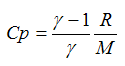
| Cp | specific heat (constant pressure) | Z | compressibility |
| r | density | g | Cp/Cv |
| G | mass flux | Â | Â |
Analysis One
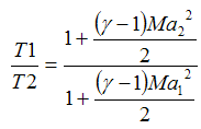
This analysis derives the
relationship between the stagnation temperature, flowing temperature,
and the Mach number for a flowing ideal gas. Stagnation temperature is
the temperature a flowing gas rises to when it is brought isentropically
to rest, thereby converting its kinetic energy into enthalpy.Conservation of energy requires that the energy balances:
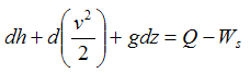 | Eq. (1) |
 | Eq. (2) |
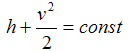
The gas, at rest, has no kinetic energy and is at its stagnation temperature (Tst), while the moving gas has kinetic energy and is at another temperature (T). The energies are therefore:
energy at rest, per unit mass = 0 + Cp Tstenergy in motion, per unit mass = v2/2 + Cp T
Equating the energy at rest and in motion:
| hst= h+v2/2 | Eq. (3) |
| h= hst-v2/2 | Eq. (4) |
 | Eq. (5) |
- Stagnation enthalpy of the fluid during adiabatic flow is constant. For an ideal gas, this implies the stagnation temperature is constant.
- Enthalpy of the gas drops and kinetic energy increases in the direction of flow.
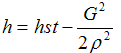
- For as given mass flux the enthalpy and density are related to each other.
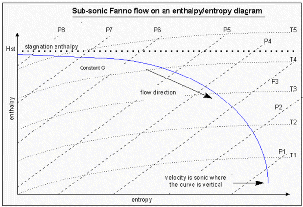 |
| Figure 1: Sub-sonic Flanno Flow |
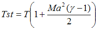
| Cp Tst = v2/2 + Cp T | Eq. (6) |
Also for an ideal gas:
 | Eq. (7) |
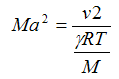 | Eq. (8) |
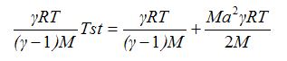 | Eq. (9) |
 | Eq. (10) |
If the gas is flowing adiabatically, then no energy has been added or subtracted from it and Tst is constant along the length of the pipe. Knowing Tst, then the above equation can be used to find the flowing temperature from the Mach number, (or vice versa) at any position along the pipe.
Analysis Two
This analysis uses the principles
of conservation of energy and mass to derive a relationship between
pressure and Mach number at up and downstream conditions, for adiabatic
flow in a pipe of constant cross-sectional area.The conservation of mass requires the mass flux to be the same at any position along a pipe. Mass flux at any of these positions can be expressed in terms of density and velocity :
| Eq. (11) |
 | Eq. (12) |
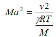 | Eq. (13) |
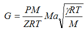 | Eq. (14) |
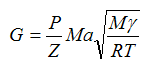 | Eq. (15) |
 | Eq. (16) |
Â
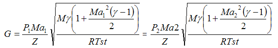 | Eq. (17) |
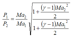 | Eq. (18) |
 | Eq. (19) |
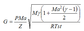
Analysis Three
Now the
momentum equation is introduced to incorporates the losses due to
friction. The derivation is available in any standard textbook for
compressible flow In summary the final result is: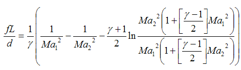 | Eq. (20) |
f= Average Darcy friction factor
L= Equivalent length of line
d= I.D. of the line
Thus this equation relates losses due to friction to inlet and outlet velocities. Solving for the unknown parameter requires a trial and error approach and is suitable for an Excel spreadsheet using the "Goal Seek" or "Solver" tools. Depending on the number of unknowns one or all three of the following equations need to be solved simultaneously:
Mass balance Equation 11
Energy balance Equation18 or 19
Momentum balance Equation 20.
In cases where the outlet velocity is defined as Mach 1, then the equation can be solved for the maximum length, which can be used to flow a certain amount of fluid through a line of known diameter. Beyond this length choked flow condition occurs and, as explained above, any further increase in pipe length will cause the flow to decrease in such a manner that velocity at the end of the pipe is still sonic ( Mach=1). This particular application is of considerable practical use in sizing blowdown lines or relief valve outlet lines relieving to the atmosphere.
Recall that the above equations have assumed that the gas is ideal. One can compensate for non-ideality to an extent by incorporating the Z factor. A rigorous approach implies solving simultaneously the momentum, energy, and mass balance equation numerically. An analytical approach, as given above for ideal gases, is useful most of the time and the results are valid for engineering purpose.
Isothermal Flow
In isothermal flow, the temperature of the gas remains constant. This simplifies matters considerably. Starting with the mechanical energy equation:
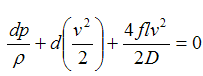 | Eq. (21) |
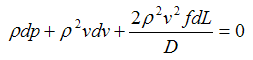 | Eq. (22) |
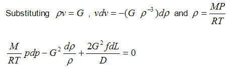 | Eq. (23) |
Rearranging and integrating gives:
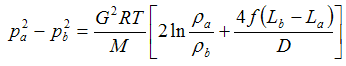 | Eq. (24) |
When
the temperature change over the conduit is small Equation 24 can be
used instead of the adiabatic Equation 20. Adibatic flow below Mach
0.3 follows Equation 24 closely.
If Equation 24 is differentiated with respect to ?b  to obtain a maximum G then:
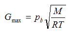 | Eq. (25) |
and the exit Mach number is:
 | Eq. (26) |
This
apparent choking condition for isothermal flow is not physically
meaningful, as at these high speeds, and rates of expansion, isothermal
conditions are not possible.
References
- Unit operations of Chemical Engineering- Mccabe, Smith and Hariott; McGraw-Hill
No comments:
Post a Comment